Chapter 1: The Thrill of the 100 Meter Sprint

The excitement of the Summer Olympics may have concluded, but the fascinating physics of events like the men's 100 meter sprint continues. If you caught the race, you know how incredibly tight it was. Noah Lyles secured the gold medal with a time that edged out Kishane Thompson by a mere 0.005 seconds. In a way, that feels almost like a tie, and both athletes deserve recognition.

Now, wouldn’t it be intriguing to examine the relationship between speed and time for these sprinters? Absolutely! However, acquiring such data can be a challenge. While I’m sure detailed statistics exist, I’ll have to rely on information I can locate online. Although there’s a video of the race, it doesn't provide the positional data over time that one might gather through video analysis.

But hold on! I stumbled upon an excellent video featuring data from Ashton Eaton. Let’s take a look.

This video offers insights, albeit it's not the primary source for the data. It displays the velocities of each runner at the 30 and 60-meter marks along with their maximum speeds. Unfortunately, it lacks specific timing for these velocities, and we only have two key points. It would be ideal to have velocity readings at every 10-meter interval.

No worries! I will start with the split times sourced from Reddit. Below is a graph that illustrates the position over time for lane 2, though similar trends can be observed across all lanes.

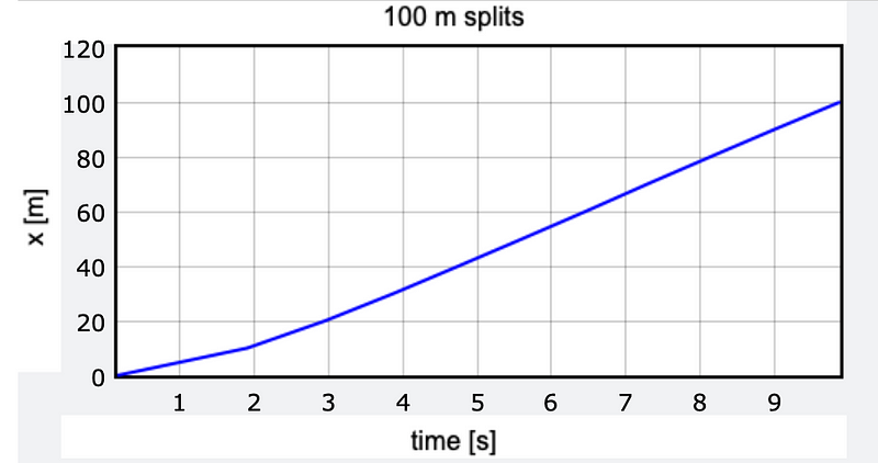
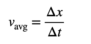
The data suggests a brief acceleration phase followed by a steady velocity. However, we can refine our analysis. By knowing the time at each distance, I can calculate the average speed during the respective time intervals.

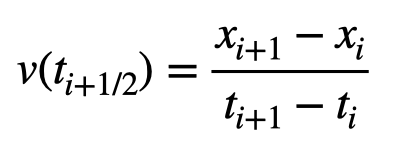
But how do we associate this average speed with the time? We can link the average speed to the midpoint of each time interval. If I have times ( t_i ) at positions ( x_i ) (where ( i ) is 0, 1, 2...), I can express a velocity-time function.

Now we can visualize this velocity at the newly calculated time points. Additionally, I can start with a data point indicating a velocity of 0 m/s at a reaction time of 0.178 seconds for Lyles. Incorporating data points from the Ashton Eaton video gives us three velocities (start, at 30 meters, and at 60 meters), plus a fourth derived from the final race time and an estimated last velocity. Here's what the data looks like now.

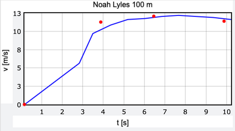
While the speed initially appears a bit irregular, it aligns reasonably well with the velocity data from the other video. This is the best approximation I can achieve for now, pending better data.

Chapter 2: Modeling the 100 Meter Sprint

Physicists are inclined to create models based on observed data. When we analyze velocity-time data, we often seek a mathematical representation. One traditional approach is the Keller model of running, which posits that a runner moves under a consistent driving force while contending with a drag force that depends on their speed. The representation of a runner's speed can be expressed mathematically as follows:

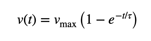
It's important to note that this is purely a mathematical abstraction. It doesn't imply that drag forces operate linearly; rather, it suggests a reason why runners may not continue accelerating. Additionally, this model assumes that runners achieve a maximum speed without gradually slowing down. More recent models do exist that account for this variation, but for now, let’s proceed with this one.

Below is a comparison of this model plotted alongside the velocity data derived from the split times. I will utilize a maximum speed of 12 m/s and a time constant of ( tau = 1.09 ) seconds, shifting the velocity data slightly to account for the runner starting just after ( t = 0 ).

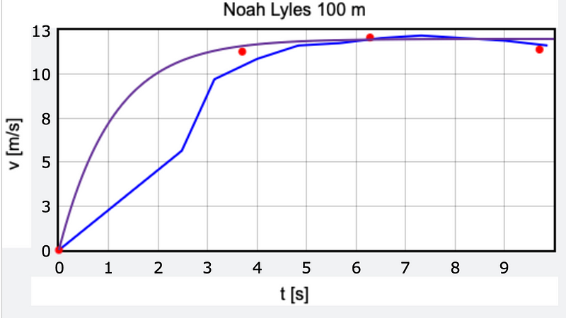
While it's not a perfect correlation, it’s still quite reasonable.

However, I have an even more effective model for human running, which I like to refer to as the "bouncing ball" model. This concept suggests that as a runner pushes off the ground, they momentarily experience a projectile motion similar to a ball. During this airborne phase, the runner maneuvers their legs in a cyclical motion.

To initiate this upward motion, a force must be applied at the ground's surface during the runner's impact. This "bouncing ball" dynamic allows for an increase in speed, but the force exerted by the runner is finite, and the time spent in contact with the ground diminishes as speed increases. Ultimately, there comes a point where the runner only exerts upward force, ceasing to accelerate.

Here’s a visual representation of this model (the full Python code for this animation is available).

I believe this model offers a better fit than the Keller model. Let’s see if we can align this bouncing ball model with Noah Lyles' performance. There are two adjustable parameters: the duration it takes for the legs to alternate and the maximum force the runner can exert. By fine-tuning these values, I can achieve a satisfactory fit. Here’s what I found.

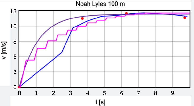
The magenta "stair step" curve represents the bouncing ball model. Notice that during the airborne phase, the horizontal velocity remains unchanged, only altering during ground contact. While the data appears to fit well, further refinement is required; my "in-air" time of 0.47 seconds seems excessive for an Olympic athlete, though it certainly is visually engaging.

Homework

Yes, there is some homework! Try to derive a reasonable estimate for the airborne duration for Noah Lyles. Use this figure in my bouncing ball model (linked above) and adjust the impact force to optimize the fit. The beauty of the bouncing ball model lies in its reliance on real forces, which allows for interesting variations, such as altering the gravitational field. For instance, how would the 100 meter sprint times change if it were conducted on the moon (assuming there's air so runners don’t need space suits)?

Moreover, we could analyze the effects of air drag on these athletes. How significant is the impact of a 3 mph headwind? Lastly, gather speed-time data for all competitors in the 100m sprint and utilize Web VPython to create an engaging animation of the race. That would be an exciting project!